Machine Learning with Fianacial Time Series Classification using TensorFlow
Summarize
Time series are the lifeblood that circulates the body of finance and time series analysis is the heart that moves that fluid. That’s the way finance has always functioned and always will. However, the nature of that blood, body and heart has evolved over time. There is more data, both more sources of data (e.g. more exchanges, plus social media, plus news, etc.) and more frequent delivery of data (i.e. IOS of messages per second 10 years ago has become IOOs of 1,000s of messages per second today). More and different analysis techniques are being brought to bear. Most of the analysis techniques are not different in the sense of being new, and have their basis in statistics, but their applicability has closely followed the amount of computing power available. The growth in available computing power is faster than the growth in time series volumes and so it is possible to analyze time series today at scale in ways that weren’t tractable previously. This is particularly true of machine learning, especially deep learning, and these techniques hold great promise for time series. As time series become more dense and many time series overlap, machine learning offers a way to the signal from the noise even when the noise can see overwhelming, and deep learning holds great potential because it is often the best fit for the almost random nature of financial time series.
The Proposition
The proposition for my research is straightforward, that financial markets are increasingly global and if we follow the sun from Asia to Europe to the US and so on we can use information from an earlier timezone to our advantage in a later timezone.
Financial markets are increasingly global and if we follow the sun from Asia to Europe to the US and so on we can use information from an earlier timezone to our advantage in a later timezone.
The table below shows a number of stock market indices from around the globe, their closing times in EST, and the delay in hours between the close that index and the close of the S&P 500 in New York (hence taking EST as a base timezone). For example, Australian markets close for the day 15 hours before US markets close. So, if the close of the All Ords in Australia is a useful predictor of the close of the S&P 500 for a given day we can use that information to guide our trading activity. Continuing our example of the Australian All Ords, if this index closes up and we think that means the S&P 500 will close up as well then we should buy either stocks that compose the S&P 500 or more likely an ETF that tracks the S&P 500.
| Index | Country | Closing Time (EST) | Hours Before S&P Close |
|---|---|---|---|
| All Ords | Australia | 0100 | 15 |
| Nikkei 225 | Japan | 0200 | 14 |
| Hang Seng | Hong Kong | 0400 | 12 |
| DAX | Germany | 1130 | 4.5 |
| FTSE 100 | UK | 1130 | 4.5 |
| NYSE Composite | US | 1600 | 0 |
| Dow Jones Industrial Average | US | 1600 | 0 |
| S&P 500 | US | 1600 | 0 |
Setup
First let’s import necessary libraries.
!pip install https://storage.googleapis.com/tensorflow/linux/cpu/tensorflow-0.5.0-cp27-none-linux_x86_64.whl
Downloading/unpacking https://storage.googleapis.com/tensorflow/linux/cpu/tensorflow-0.5.0-cp27-none-linux_x86_64.whl
  Downloading tensorflow-0.5.0-cp27-none-linux_x86_64.whl (10.9MB): 10.9MB downloaded
Requirement already satisfied (use --upgrade to upgrade): numpy>=1.9.2 in /usr/local/lib/python2.7/dist-packages (from tensorflow==0.5.0)
Downloading/unpacking six>=1.10.0 (from tensorflow==0.5.0)
  Downloading six-1.10.0-py2.py3-none-any.whl
Installing collected packages: tensorflow, six
  Found existing installation: six 1.8.0
    Not uninstalling six at /usr/lib/python2.7/dist-packages, owned by OS
Successfully installed tensorflow six
Cleaning up...
import StringIO

import pandas as pd
from pandas.tools.plotting import autocorrelation_plot
from pandas.tools.plotting import scatter_matrix

import numpy as np

import matplotlib.pyplot as plt

import gcp
import gcp.bigquery as bq

import tensorflow as tf
Get the Data
We’ll use data from the last 5 years (approximately) - 1/1/2012-10/1/2017 - for the S&P 500 (S&P), NYSE, Dow Jones Industrial Average (DJIA), Nikkei 225 (Nikkei), Hang Seng, FTSE 100 (FTSE), DAX, All Ordinaries (AORD) indices.
We’ll use the built-in connector functionality in Cloud Datalab to access this data as Pandas DataFrames.
%%sql --module market_data_query
SELECT * FROM $market_data_table
snp = bq.Query(market_data_query, market_data_table=bq.Table('bingo-ml-1:market_data.snp')).to_dataframe().set_index('Date')
nyse = bq.Query(market_data_query, market_data_table=bq.Table('bingo-ml-1:market_data.nyse')).to_dataframe().set_index('Date')
djia = bq.Query(market_data_query, market_data_table=bq.Table('bingo-ml-1:market_data.djia')).to_dataframe().set_index('Date')
nikkei = bq.Query(market_data_query, market_data_table=bq.Table('bingo-ml-1:market_data.nikkei')).to_dataframe().set_index('Date')
hangseng = bq.Query(market_data_query, market_data_table=bq.Table('bingo-ml-1:market_data.hangseng')).to_dataframe().set_index('Date')
ftse = bq.Query(market_data_query, market_data_table=bq.Table('bingo-ml-1:market_data.ftse')).to_dataframe().set_index('Date')
dax = bq.Query(market_data_query, market_data_table=bq.Table('bingo-ml-1:market_data.dax')).to_dataframe().set_index('Date')
aord = bq.Query(market_data_query, market_data_table=bq.Table('bingo-ml-1:market_data.aord')).to_dataframe().set_index('Date')
Pre-process Data
Preprocessing the data is quite straightforward in the first instance. I’m interested in closing prices so for convenience I’ll extract the closing prices for each of the indices into a single Pandas DataFrame, called closing_data. Because not all of the indices have the same number of values, mainly due to bank holidays, I’ll forward fill the gaps. This simply means that if a values isn’t available for day N we’ll fill it with the value for day N-1 (or N-2 etc.) such that we fill it with the latest available value.
closing_data = pd.DataFrame()

closing_data['snp_close'] = snp['Close']
closing_data['nyse_close'] = nyse['Close']
closing_data['djia_close'] = djia['Close']
closing_data['nikkei_close'] = nikkei['Close']
closing_data['hangseng_close'] = hangseng['Close']
closing_data['ftse_close'] = ftse['Close']
closing_data['dax_close'] = dax['Close']
closing_data['aord_close'] = aord['Close']

# Pandas includes a very convenient function for filling gaps in the data.
closing_data = closing_data.fillna(method='ffill')
About the data we have sourced
Well, so far, I’ve sourced five years of time series for eight financial indices, combined the pertinent data into a single data structure and harmonized the data to have the same number of entries in 20 lines of code in this notebook.
Exploratory Data Analysis
Exploratory Data Analysis (EDA) is foundational to my work with machine learning (and any other sort of analysis). EDA means getting to know your data, getting your fingers dirty with your data, feeling it and seeing it. The end result is that data is your friend and you know it like you know a friend, so when you build models you build them based on an actual, practical, physical understanding of the data and not assumptions of vaguely held notions. EDA means you will understand your assumptions and why you’re making those assumptions.
closing_data.describe()
| snp_close | nyse_close | djia_close | nikkei_close | hangseng_close | ftse_close | dax_close | aord_close | |
|---|---|---|---|---|---|---|---|---|
| count | 1447.000000 | 1447.000000 | 1447.000000 | 1447.000000 | 1447.000000 | 1447.000000 | 1447.000000 | 1447.000000 |
| mean | 1549.733275 | 8920.468489 | 14017.464990 | 12529.915089 | 22245.750485 | 6100.506356 | 7965.888030 | 4913.770143 |
| std | 338.278280 | 1420.830375 | 2522.948044 | 3646.022665 | 2026.412936 | 553.389736 | 1759.572713 | 485.052575 |
| min | 1022.580017 | 6434.810059 | 9686.480469 | 8160.009766 | 16250.269531 | 4805.799805 | 5072.330078 | 3927.600098 |
| 25% | 1271.239990 | 7668.234863 | 11987.635254 | 9465.930176 | 20841.259765 | 5677.899902 | 6457.090088 | 4500.250000 |
| 50% | 1433.189941 | 8445.769531 | 13323.360352 | 10774.150391 | 22437.439453 | 6008.899902 | 7435.209961 | 4901.100098 |
| 75% | 1875.510010 | 10370.324707 | 16413.575196 | 15163.069824 | 23425.334961 | 6622.650147 | 9409.709961 | 5346.150147 |
| max | 2130.820068 | 11239.660156 | 18312.390625 | 20868.029297 | 28442.750000 | 7104.000000 | 12374.730469 | 5954.799805 |
We can see that the various indices operate on scales differing by orders of magnitude it just means we’ll scale our data so that - for example - operations involving multiple indices are not unduly influenced by a single, massive index.
Let’s plot out data.
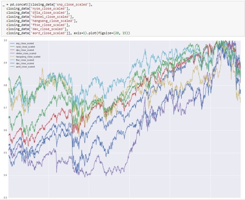
As expected the structure isn’t uniformly visible for the indices so let’s scale the value for each day of a given index divided by the maximum value for that index in the dataset and replot (i.e. the maximum value of all indicies will be 1).
closing_data['snp_close_scaled'] = closing_data['snp_close'] / max(closing_data['snp_close'])
closing_data['nyse_close_scaled'] = closing_data['nyse_close'] / max(closing_data['nyse_close'])
closing_data['djia_close_scaled'] = closing_data['djia_close'] / max(closing_data['djia_close'])
closing_data['nikkei_close_scaled'] = closing_data['nikkei_close'] / max(closing_data['nikkei_close'])
closing_data['hangseng_close_scaled'] = closing_data['hangseng_close'] / max(closing_data['hangseng_close'])
closing_data['ftse_close_scaled'] = closing_data['ftse_close'] / max(closing_data['ftse_close'])
closing_data['dax_close_scaled'] = closing_data['dax_close'] / max(closing_data['dax_close'])
closing_data['aord_close_scaled'] = closing_data['aord_close'] / max(closing_data['aord_close'])
Now we see that over the five year period these indices are correlated (i.e. sudden drops from economic events happened globally to all indices, general rises otherwise). Let’s plot autocorrelations for each of the indicies (correlations of the index with lagged values of the index, e.g. is yesterday indicative of today?)
fig = plt.figure()
fig.set_figwidth(20)
fig.set_figheight(15)

_ = autocorrelation_plot(closing_data['snp_close'], label='snp_close')
_ = autocorrelation_plot(closing_data['nyse_close'], label='nyse_close')
_ = autocorrelation_plot(closing_data['djia_close'], label='djia_close')
_ = autocorrelation_plot(closing_data['nikkei_close'], label='nikkei_close')
_ = autocorrelation_plot(closing_data['hangseng_close'], label='hangseng_close')
_ = autocorrelation_plot(closing_data['ftse_close'], label='ftse_close')
_ = autocorrelation_plot(closing_data['dax_close'], label='dax_close')
_ = autocorrelation_plot(closing_data['aord_close'], label='aord_close')

plt.legend(loc='upper right')
<matplotlib.legend.Legend at 0x7fbd0ded76d0>
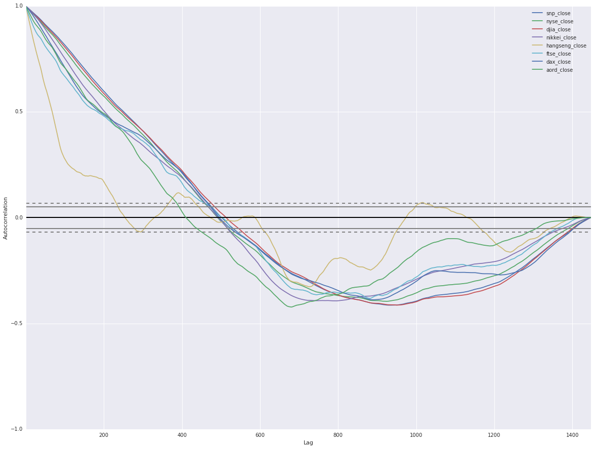
We see strong autocorrelations, positive for ~500 lagged days then going negative. This tells us if an index is rising it tends to carry on rising and vice versa. This is showing that we are on the right path with index data.
Next we’ll look at a scatter matix (i.e. everything plotted against everything) to see how indicies are correlated with each other.
_ = scatter_matrix(pd.concat([closing_data['snp_close_scaled'],
  closing_data['nyse_close_scaled'],
  closing_data['djia_close_scaled'],
  closing_data['nikkei_close_scaled'],
  closing_data['hangseng_close_scaled'],
  closing_data['ftse_close_scaled'],
  closing_data['dax_close_scaled'],
  closing_data['aord_close_scaled']], axis=1), figsize=(20, 20), diagonal='kde')
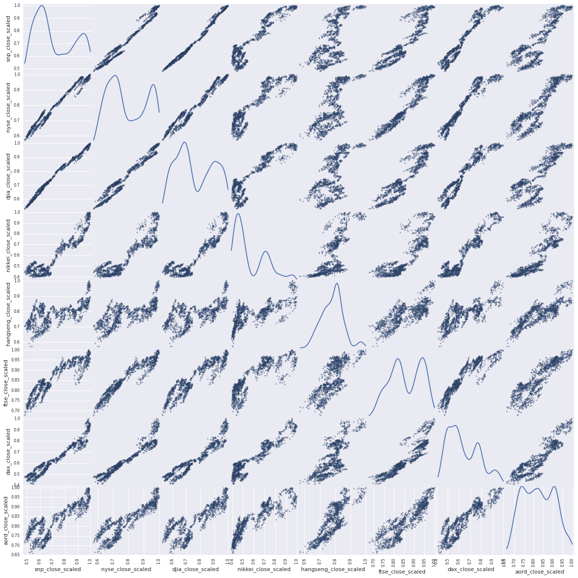
Significant correlations across the board. Further evidence that my proposition is workable and one market is influenced by another. The process we’re following of gradual incremental experimentation and progress is spot on what we should be doing.
we’re getting there…
The actual value of an index is not that useful to us for modeling. It’s indicative, it’s useful - and we’ve seen that from our visualizations to date - but to really get to the aim we’re looking for we need a time series that is stationary in the mean (i.e. there is no trend in the data). There are various ways of doing that but they all essentially look the the difference between values rather than the absolute value. In the case of market data the usual practice is to work with logged returns (the natural logaritm of the index today divided by the index yesterday). I.e.
ln(Vt/Vt-1)
Where Vt is the value of the index on day t and Vt-1 is the value of the index on day t-1. There are other reasons why the log return is prefereable to the percent return (for example the log is normally distributed and additive) and we get to a stationary time series.
Let’s calculate the log returns and plot those. I’ll do this in a new DataFrame.
log_return_data = pd.DataFrame()

log_return_data['snp_log_return'] = np.log(closing_data['snp_close']/closing_data['snp_close'].shift())
log_return_data['nyse_log_return'] = np.log(closing_data['nyse_close']/closing_data['nyse_close'].shift())
log_return_data['djia_log_return'] = np.log(closing_data['djia_close']/closing_data['djia_close'].shift())
log_return_data['nikkei_log_return'] = np.log(closing_data['nikkei_close']/closing_data['nikkei_close'].shift())
log_return_data['hangseng_log_return'] = np.log(closing_data['hangseng_close']/closing_data['hangseng_close'].shift())
log_return_data['ftse_log_return'] = np.log(closing_data['ftse_close']/closing_data['ftse_close'].shift())
log_return_data['dax_log_return'] = np.log(closing_data['dax_close']/closing_data['dax_close'].shift())
log_return_data['aord_log_return'] = np.log(closing_data['aord_close']/closing_data['aord_close'].shift())

log_return_data.describe()
| snp_log_return | nyse_log_return | djia_log_return | nikkei_log_return | hangseng_log_return | ftse_log_return | dax_log_return | aord_log_return | |
|---|---|---|---|---|---|---|---|---|
| count | 1446.000000 | 1446.000000 | 1446.000000 | 1446.000000 | 1446.000000 | 1446.000000 | 1446.000000 | 1446.000000 |
| mean | 0.000366 | 0.000203 | 0.000297 | 0.000352 | -0.000032 | 0.000068 | 0.000313 | 0.000035 |
| std | 0.010066 | 0.010538 | 0.009287 | 0.013698 | 0.011779 | 0.010010 | 0.013092 | 0.009145 |
| min | -0.068958 | -0.073116 | -0.057061 | -0.111534 | -0.060183 | -0.047798 | -0.064195 | -0.042998 |
| 25% | -0.004048 | -0.004516 | -0.003943 | -0.006578 | -0.005875 | -0.004863 | -0.005993 | -0.004767 |
| 50% | 0.000628 | 0.000551 | 0.000502 | 0.000000 | 0.000000 | 0.000208 | 0.000740 | 0.000406 |
| 75% | 0.005351 | 0.005520 | 0.005018 | 0.008209 | 0.006169 | 0.005463 | 0.006807 | 0.005499 |
| max | 0.046317 | 0.051173 | 0.041533 | 0.074262 | 0.055187 | 0.050323 | 0.052104 | 0.034368 |
Looking at log returns we’re now moving forward more rapidly. The mean, min, max are all similar. I can go further and center the series on zero, scale them and normalize the standard deviation but there’s no need to do that at this point. Let’s move forward and iterate if necessary.
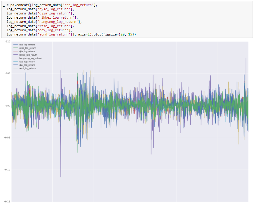
We can see from this that the log returns of our indices are similarly scaled and centered with no trend visible in the data. Looking good, now let’s look at autocorrelations.
fig = plt.figure()
fig.set_figwidth(20)
fig.set_figheight(15)

_ = autocorrelation_plot(log_return_data['snp_log_return'], label='snp_log_return')
_ = autocorrelation_plot(log_return_data['nyse_log_return'], label='nyse_log_return')
_ = autocorrelation_plot(log_return_data['djia_log_return'], label='djia_log_return')
_ = autocorrelation_plot(log_return_data['nikkei_log_return'], label='nikkei_log_return')
_ = autocorrelation_plot(log_return_data['hangseng_log_return'], label='hangseng_log_return')
_ = autocorrelation_plot(log_return_data['ftse_log_return'], label='ftse_log_return')
_ = autocorrelation_plot(log_return_data['dax_log_return'], label='dax_log_return')
_ = autocorrelation_plot(log_return_data['aord_log_return'], label='aord_log_return')

plt.legend(loc='upper right')
<matplotlib.legend.Legend at 0x7fbd0b66d050>
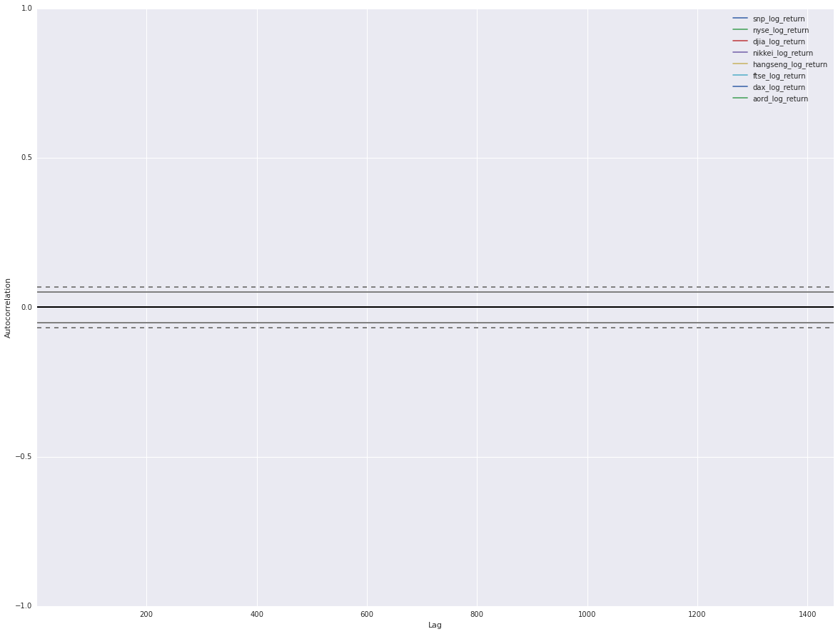
No autocorrelations visible on the plot which is what we’re looking for. Individual financial markets are Markov processes, knowledge of history doesn’t allow you to predict the future. We have time series for our indicies that are stationary in the mean, similarly centered and scaled. Now let’s start to look for signals to predict the close of the S&P 500.
Let’s look at a scatter plot to see how our log return indices correlate with each other.
_ = scatter_matrix(log_return_data, figsize=(20, 20), diagonal='kde')
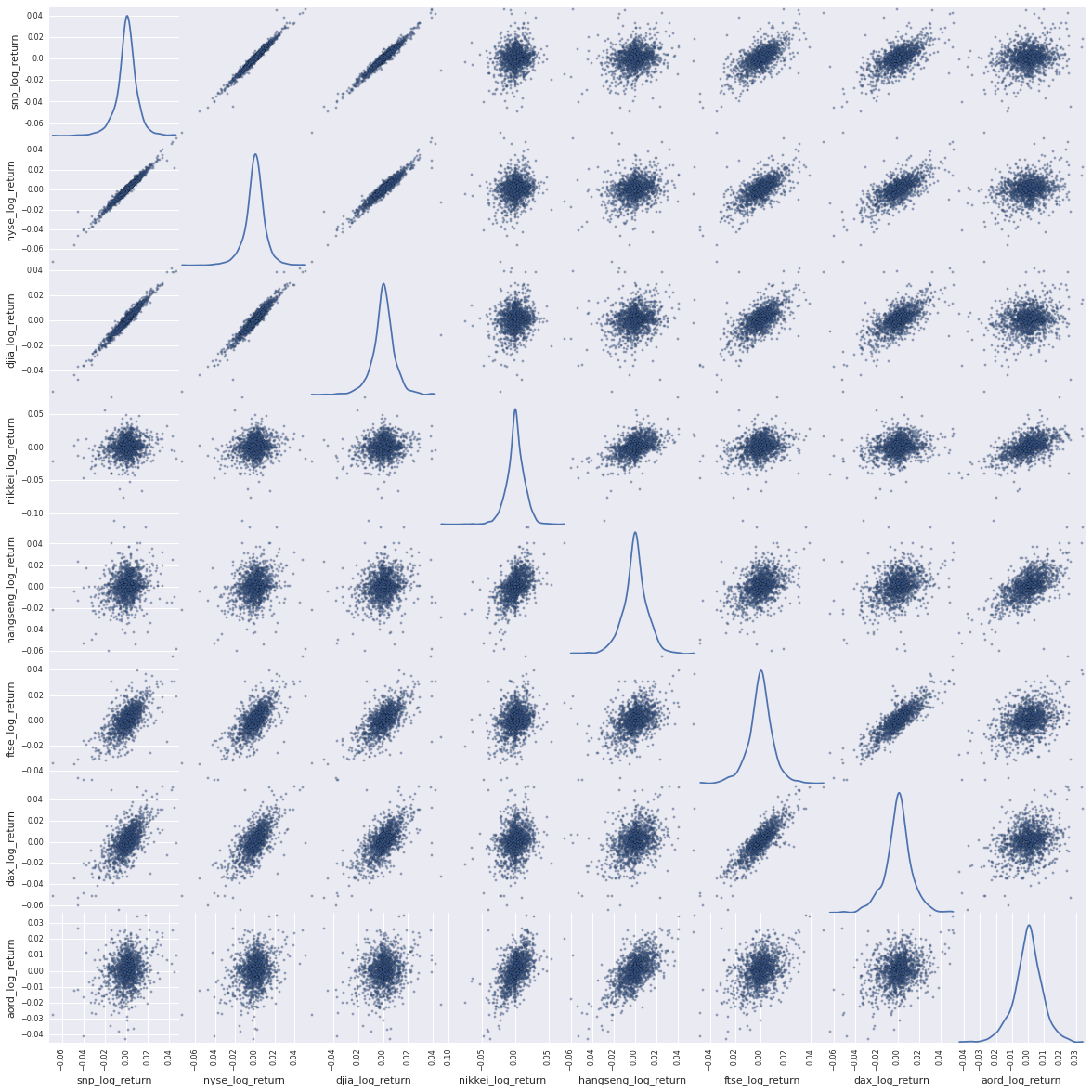
The story with our scatter plot above for log returns is more subtle and more insightful. The US indices are strongly correlated. The other indices less so, also expected, but there is structure and signal there.
Now let’s start to quantify it so we can start to choose features for our model.
First let’s look at how the log returns for the S&P 500 close correlate with other indices closes available on the same day.
tmp = pd.DataFrame()
tmp['snp_0'] = log_return_data['snp_log_return']
tmp['nyse_1'] = log_return_data['nyse_log_return'].shift()
tmp['djia_1'] = log_return_data['djia_log_return'].shift()
tmp['nikkei_0'] = log_return_data['nikkei_log_return']
tmp['hangseng_0'] = log_return_data['hangseng_log_return']
tmp['ftse_0'] = log_return_data['ftse_log_return']
tmp['dax_0'] = log_return_data['dax_log_return']
tmp['aord_0'] = log_return_data['aord_log_return']
tmp.corr().icol(0)
snp_0         1.000000
nyse_1       -0.038903
djia_1       -0.047759
nikkei_0      0.151892
hangseng_0    0.205776
ftse_0        0.656523
dax_0         0.654757
aord_0        0.227845
Name: snp_0, dtype: float64
Here I’m directly working with our proposition. correlating the close of the S&P 500 with signals available before the close of the S&P 500. Et voila! The S&P 500 close is correlated with European indices (~0.65 for the FTSE and DAX) which is a strong correlation and Asian/Oceanian indices (~0.15-0.22) which is a significant correlation, but not with US indicies. We have available signals from other indicies and regions for our model.
Now let’s look a how the log returns for the S&P close correlate with index values from the previous day. Following from the proposition that financial markets are Markov processes there should be little or no value in hostorical values.
tmp = pd.DataFrame()
tmp['snp_0'] = log_return_data['snp_log_return']
tmp['nyse_1'] = log_return_data['nyse_log_return'].shift(2)
tmp['djia_1'] = log_return_data['djia_log_return'].shift(2)
tmp['nikkei_0'] = log_return_data['nikkei_log_return'].shift()
tmp['hangseng_0'] = log_return_data['hangseng_log_return'].shift()
tmp['ftse_0'] = log_return_data['ftse_log_return'].shift()
tmp['dax_0'] = log_return_data['dax_log_return'].shift()
tmp['aord_0'] = log_return_data['aord_log_return'].shift()
tmp.corr().icol(0)
snp_0         1.000000
nyse_1        0.043572
djia_1        0.030391
nikkei_0      0.010357
hangseng_0    0.040744
ftse_0        0.012052
dax_0         0.006265
aord_0        0.021371
Name: snp_0, dtype: float64
We see little to no correlation in this data meaning that yesterday’s values are no practical help in predicting today’s close. Let’s go one step further and look at correlations between today the the day before yesterday.
tmp = pd.DataFrame()
tmp['snp_0'] = log_return_data['snp_log_return']
tmp['nyse_1'] = log_return_data['nyse_log_return'].shift(3)
tmp['djia_1'] = log_return_data['djia_log_return'].shift(3)
tmp['nikkei_0'] = log_return_data['nikkei_log_return'].shift(2)
tmp['hangseng_0'] = log_return_data['hangseng_log_return'].shift(2)
tmp['ftse_0'] = log_return_data['ftse_log_return'].shift(2)
tmp['dax_0'] = log_return_data['dax_log_return'].shift(2)
tmp['aord_0'] = log_return_data['aord_log_return'].shift(2)

tmp.corr().icol(0)
snp_0         1.000000
nyse_1       -0.070845
djia_1       -0.071228
nikkei_0     -0.015766
hangseng_0   -0.031368
ftse_0        0.017085
dax_0        -0.005546
aord_0        0.004254
Name: snp_0, dtype: float64
Again, little to no correlations.
At this point I’ve done a good research on exploratory data analysis. Visualized our data, got to know it, felt the quality of the fabric as it were. I’ve tranformed into a form that is useful for modelling - log returns in our case - and looked at how indicies relate to each other. We’ve seen that indicies from other Europe strongly correlate with US indicies, and that indicies from Asia/Oceania significantly correlate with those same indicies for a given day. Also, if we look at historical values they do not correlate with today’s values. Summing up:
** European indices from the same day are a strong predictor for the S&P 500 close.**
** Asian/Oceanian indicies from the same day are a significant predictor for the S&P 500 close.**
** Indicies from previous days are not good predictors for the S&P close.**
Feature Selection
we can now see a model:
- I can now predict whether the S&P 500 close today will be higher or lower than yesterday.
- I’ll use all our data sources - NYSE, DJIA, Nikkei, Hang Seng, FTSE, DAX, AORD.
- I’ll use 3 sets of data points - T, T-1, T-2 - where we take the data available on day T (or T-n) i.e. today’s non-US data and yesterdays US data.
Predicting whether the log return of the S&P 500 is positive or negative is a classification problem. That is, to choose one option from a finite set of options, in this case positive of negative. This is the base case of classification where only two values to choose from, known as binary classification (or logistic regression).
This includes the output of exploratory data analysis, namely that indicies from other regions on a given day influence the close of the S&P 500, and it also includes other features, the same region and previous days’ data. There are two reasons for this: One, adding some additional features to our model for the purpose of this solution to see how things perform, and two, machine learning models are very good at finding weak signals from data.
I’ll incrementally add, subtract and tweak features until I’ve got to a model till at its picking point.
In machine learning, as in most things, there are subtle tradeoffs happening but in general good data is better than good algorithms is better than good frameworks.
TensorFlow
TensorFlow is an open source software library, initiated by Google, for numerical computation using data flow graphs. TensorFlow is based on Google’s machine learning expertise and is the next generation framework used internally at Google for tasks such as translation and image recognition. It’s a wonderful framework for machine learning - expressive, efficient, and easy to use.
Feature Engineering for TensorFlow
Now we create training and test data, together with some supporting functions for evaluating our models, for TensorFlow.
Time series data is easy from a training/test perspective. Training data should come before test data and be consecutive (i.e. you model shouldn’t be trained on events from the future). That means random sampling or cross validation don’t apply to time series data. Decide on a training versus test split and divide your data into training and test datasets.
I’ll create our features together with two additional columns, ‘snp_log_return_positive’ that is 1 if the log return of the S&P 500 close is positive and 0 otherwise, and ‘snp_log_return_negative’ that is 1 if the log return of the S&P 500 close is negative and 1 otherwise. Now, logically we could encode this information in one column, ‘snp_log_return’ which is 1 if positive and 0 if negative but that’s not the way TensorFlow works for classification models. TensorFlow uses the general definition of classification (i.e. there can be many different potential values to choose from) and a form or encoding for these options called one-hot encoding. One-hot encoding means that each choice is an entry in an array and the actual value has an entry of 1 with all other values being 0. This is for the input of the model, where you categorically know which value is correct. A variation of this is used for the output, each entry in the array contains the probability of the answer being that choice. Then choose the most likely value by choosing the highest probability, together with having a measure of the confidence which can place in that answer realtive to other answers.
I’ll use 80% of our data for training and 20% for testing.
log_return_data['snp_log_return_positive'] = 0
log_return_data.ix[log_return_data['snp_log_return'] >= 0, 'snp_log_return_positive'] = 1
log_return_data['snp_log_return_negative'] = 0
log_return_data.ix[log_return_data['snp_log_return'] < 0, 'snp_log_return_negative'] = 1

training_test_data = pd.DataFrame(
  columns=[
    'snp_log_return_positive', 'snp_log_return_negative',
    'snp_log_return_1', 'snp_log_return_2', 'snp_log_return_3',
    'nyse_log_return_1', 'nyse_log_return_2', 'nyse_log_return_3',
    'djia_log_return_1', 'djia_log_return_2', 'djia_log_return_3',
    'nikkei_log_return_0', 'nikkei_log_return_1', 'nikkei_log_return_2',
    'hangseng_log_return_0', 'hangseng_log_return_1', 'hangseng_log_return_2',
    'ftse_log_return_0', 'ftse_log_return_1', 'ftse_log_return_2',
    'dax_log_return_0', 'dax_log_return_1', 'dax_log_return_2',
    'aord_log_return_0', 'aord_log_return_1', 'aord_log_return_2'])

for i in range(7, len(log_return_data)):
  snp_log_return_positive = log_return_data['snp_log_return_positive'].ix[i]
  snp_log_return_negative = log_return_data['snp_log_return_negative'].ix[i]
  snp_log_return_1 = log_return_data['snp_log_return'].ix[i-1]
  snp_log_return_2 = log_return_data['snp_log_return'].ix[i-2]
  snp_log_return_3 = log_return_data['snp_log_return'].ix[i-3]
  nyse_log_return_1 = log_return_data['nyse_log_return'].ix[i-1]
  nyse_log_return_2 = log_return_data['nyse_log_return'].ix[i-2]
  nyse_log_return_3 = log_return_data['nyse_log_return'].ix[i-3]
  djia_log_return_1 = log_return_data['djia_log_return'].ix[i-1]
  djia_log_return_2 = log_return_data['djia_log_return'].ix[i-2]
  djia_log_return_3 = log_return_data['djia_log_return'].ix[i-3]
  nikkei_log_return_0 = log_return_data['nikkei_log_return'].ix[i]
  nikkei_log_return_1 = log_return_data['nikkei_log_return'].ix[i-1]
  nikkei_log_return_2 = log_return_data['nikkei_log_return'].ix[i-2]
  hangseng_log_return_0 = log_return_data['hangseng_log_return'].ix[i]
  hangseng_log_return_1 = log_return_data['hangseng_log_return'].ix[i-1]
  hangseng_log_return_2 = log_return_data['hangseng_log_return'].ix[i-2]
  ftse_log_return_0 = log_return_data['ftse_log_return'].ix[i]
  ftse_log_return_1 = log_return_data['ftse_log_return'].ix[i-1]
  ftse_log_return_2 = log_return_data['ftse_log_return'].ix[i-2]
  dax_log_return_0 = log_return_data['dax_log_return'].ix[i]
  dax_log_return_1 = log_return_data['dax_log_return'].ix[i-1]
  dax_log_return_2 = log_return_data['dax_log_return'].ix[i-2]
  aord_log_return_0 = log_return_data['aord_log_return'].ix[i]
  aord_log_return_1 = log_return_data['aord_log_return'].ix[i-1]
  aord_log_return_2 = log_return_data['aord_log_return'].ix[i-2]
  training_test_data = training_test_data.append(
    {'snp_log_return_positive':snp_log_return_positive,
    'snp_log_return_negative':snp_log_return_negative,
    'snp_log_return_1':snp_log_return_1,
    'snp_log_return_2':snp_log_return_2,
    'snp_log_return_3':snp_log_return_3,
    'nyse_log_return_1':nyse_log_return_1,
    'nyse_log_return_2':nyse_log_return_2,
    'nyse_log_return_3':nyse_log_return_3,
    'djia_log_return_1':djia_log_return_1,
    'djia_log_return_2':djia_log_return_2,
    'djia_log_return_3':djia_log_return_3,
    'nikkei_log_return_0':nikkei_log_return_0,
    'nikkei_log_return_1':nikkei_log_return_1,
    'nikkei_log_return_2':nikkei_log_return_2,
    'hangseng_log_return_0':hangseng_log_return_0,
    'hangseng_log_return_1':hangseng_log_return_1,
    'hangseng_log_return_2':hangseng_log_return_2,
    'ftse_log_return_0':ftse_log_return_0,
    'ftse_log_return_1':ftse_log_return_1,
    'ftse_log_return_2':ftse_log_return_2,
    'dax_log_return_0':dax_log_return_0,
    'dax_log_return_1':dax_log_return_1,
    'dax_log_return_2':dax_log_return_2,
    'aord_log_return_0':aord_log_return_0,
    'aord_log_return_1':aord_log_return_1,
    'aord_log_return_2':aord_log_return_2},
    ignore_index=True)

training_test_data.describe()
| snp_log_return_positive | snp_log_return_negative | snp_log_return_1 | snp_log_return_2 | snp_log_return_3 | nyse_log_return_1 | nyse_log_return_2 | nyse_log_return_3 | djia_log_return_1 | djia_log_return_2 | ... | hangseng_log_return_2 | ftse_log_return_0 | ftse_log_return_1 | ftse_log_return_2 | dax_log_return_0 | dax_log_return_1 | dax_log_return_2 | aord_log_return_0 | aord_log_return_1 | aord_log_return_2 | |
|---|---|---|---|---|---|---|---|---|---|---|---|---|---|---|---|---|---|---|---|---|---|
| count | 1440.000000 | 1440.000000 | 1440.000000 | 1440.000000 | 1440.000000 | 1440.000000 | 1440.000000 | 1440.000000 | 1440.000000 | 1440.000000 | ... | 1440.000000 | 1440.000000 | 1440.000000 | 1440.000000 | 1440.000000 | 1440.000000 | 1440.000000 | 1440.000000 | 1440.000000 | 1440.000000 |
| mean | 0.547222 | 0.452778 | 0.000358 | 0.000346 | 0.000347 | 0.000190 | 0.000180 | 0.000181 | 0.000294 | 0.000287 | ... | -0.000056 | 0.000069 | 0.000063 | 0.000046 | 0.000326 | 0.000326 | 0.000311 | 0.000029 | 0.000011 | 0.000002 |
| std | 0.497938 | 0.497938 | 0.010086 | 0.010074 | 0.010074 | 0.010558 | 0.010547 | 0.010548 | 0.009305 | 0.009298 | ... | 0.011783 | 0.010028 | 0.010030 | 0.010007 | 0.013111 | 0.013111 | 0.013099 | 0.009153 | 0.009146 | 0.009133 |
| min | 0.000000 | 0.000000 | -0.068958 | -0.068958 | -0.068958 | -0.073116 | -0.073116 | -0.073116 | -0.057061 | -0.057061 | ... | -0.060183 | -0.047798 | -0.047798 | -0.047798 | -0.064195 | -0.064195 | -0.064195 | -0.042998 | -0.042998 | -0.042998 |
| 25% | 0.000000 | 0.000000 | -0.004068 | -0.004068 | -0.004068 | -0.004545 | -0.004545 | -0.004545 | -0.003962 | -0.003962 | ... | -0.005884 | -0.004865 | -0.004871 | -0.004871 | -0.005995 | -0.005995 | -0.005995 | -0.004774 | -0.004786 | -0.004786 |
| 50% | 1.000000 | 0.000000 | 0.000611 | 0.000611 | 0.000611 | 0.000528 | 0.000528 | 0.000528 | 0.000502 | 0.000502 | ... | 0.000000 | 0.000180 | 0.000166 | 0.000166 | 0.000752 | 0.000752 | 0.000746 | 0.000398 | 0.000384 | 0.000384 |
| 75% | 1.000000 | 1.000000 | 0.005383 | 0.005360 | 0.005360 | 0.005563 | 0.005534 | 0.005534 | 0.005023 | 0.005021 | ... | 0.006160 | 0.005472 | 0.005472 | 0.005470 | 0.006827 | 0.006827 | 0.006812 | 0.005473 | 0.005452 | 0.005452 |
| max | 1.000000 | 1.000000 | 0.046317 | 0.046317 | 0.046317 | 0.051173 | 0.051173 | 0.051173 | 0.041533 | 0.041533 | ... | 0.055187 | 0.050323 | 0.050323 | 0.050323 | 0.052104 | 0.052104 | 0.052104 | 0.034368 | 0.034368 | 0.034368 |
8 rows × 26 columns
Now let’s create our training and test data.
predictors_tf = training_test_data[training_test_data.columns[2:]]

classes_tf = training_test_data[training_test_data.columns[:2]]

training_set_size = int(len(training_test_data) * 0.8)
test_set_size = len(training_test_data) - training_set_size

training_predictors_tf = predictors_tf[:training_set_size]
training_classes_tf = classes_tf[:training_set_size]
test_predictors_tf = predictors_tf[training_set_size:]
test_classes_tf = classes_tf[training_set_size:]

training_predictors_tf.describe()
| snp_log_return_1 | snp_log_return_2 | snp_log_return_3 | nyse_log_return_1 | nyse_log_return_2 | nyse_log_return_3 | djia_log_return_1 | djia_log_return_2 | djia_log_return_3 | nikkei_log_return_0 | ... | hangseng_log_return_2 | ftse_log_return_0 | ftse_log_return_1 | ftse_log_return_2 | dax_log_return_0 | dax_log_return_1 | dax_log_return_2 | aord_log_return_0 | aord_log_return_1 | aord_log_return_2 | |
|---|---|---|---|---|---|---|---|---|---|---|---|---|---|---|---|---|---|---|---|---|---|
| count | 1152.000000 | 1152.000000 | 1152.000000 | 1152.000000 | 1152.000000 | 1152.000000 | 1152.000000 | 1152.000000 | 1152.000000 | 1152.000000 | ... | 1152.000000 | 1152.000000 | 1152.000000 | 1152.000000 | 1152.000000 | 1152.000000 | 1152.000000 | 1152.000000 | 1152.000000 | 1152.000000 |
| mean | 0.000452 | 0.000444 | 0.000451 | 0.000314 | 0.000308 | 0.000317 | 0.000382 | 0.000376 | 0.000381 | 0.000286 | ... | 0.000078 | 0.000163 | 0.000148 | 0.000153 | 0.000378 | 0.000347 | 0.000350 | 0.000087 | 0.000075 | 0.000093 |
| std | 0.010291 | 0.010286 | 0.010285 | 0.010921 | 0.010917 | 0.010916 | 0.009341 | 0.009337 | 0.009335 | 0.013828 | ... | 0.011722 | 0.009920 | 0.009918 | 0.009917 | 0.012809 | 0.012807 | 0.012807 | 0.009021 | 0.009025 | 0.009020 |
| min | -0.068958 | -0.068958 | -0.068958 | -0.073116 | -0.073116 | -0.073116 | -0.057061 | -0.057061 | -0.057061 | -0.111534 | ... | -0.058270 | -0.047792 | -0.047792 | -0.047792 | -0.064195 | -0.064195 | -0.064195 | -0.042998 | -0.042998 | -0.042998 |
| 25% | -0.004001 | -0.004001 | -0.003994 | -0.004462 | -0.004462 | -0.004415 | -0.003865 | -0.003865 | -0.003851 | -0.006914 | ... | -0.005689 | -0.004849 | -0.004852 | -0.004852 | -0.005527 | -0.005611 | -0.005611 | -0.004591 | -0.004607 | -0.004591 |
| 50% | 0.000721 | 0.000721 | 0.000725 | 0.000646 | 0.000646 | 0.000655 | 0.000561 | 0.000561 | 0.000580 | 0.000000 | ... | 0.000000 | 0.000195 | 0.000166 | 0.000195 | 0.000700 | 0.000694 | 0.000694 | 0.000433 | 0.000422 | 0.000433 |
| 75% | 0.005607 | 0.005591 | 0.005591 | 0.005922 | 0.005908 | 0.005908 | 0.005098 | 0.005071 | 0.005071 | 0.008589 | ... | 0.006406 | 0.005649 | 0.005637 | 0.005637 | 0.006712 | 0.006697 | 0.006697 | 0.005191 | 0.005191 | 0.005235 |
| max | 0.046317 | 0.046317 | 0.046317 | 0.051173 | 0.051173 | 0.051173 | 0.041533 | 0.041533 | 0.041533 | 0.055223 | ... | 0.055187 | 0.050323 | 0.050323 | 0.050323 | 0.052104 | 0.052104 | 0.052104 | 0.034368 | 0.034368 | 0.034368 |
8 rows × 24 columns
test_predictors_tf.describe()
| snp_log_return_1 | snp_log_return_2 | snp_log_return_3 | nyse_log_return_1 | nyse_log_return_2 | nyse_log_return_3 | djia_log_return_1 | djia_log_return_2 | djia_log_return_3 | nikkei_log_return_0 | ... | hangseng_log_return_2 | ftse_log_return_0 | ftse_log_return_1 | ftse_log_return_2 | dax_log_return_0 | dax_log_return_1 | dax_log_return_2 | aord_log_return_0 | aord_log_return_1 | aord_log_return_2 | |
|---|---|---|---|---|---|---|---|---|---|---|---|---|---|---|---|---|---|---|---|---|---|
| count | 288.000000 | 288.000000 | 288.000000 | 288.000000 | 288.000000 | 288.000000 | 288.000000 | 288.000000 | 288.000000 | 288.000000 | ... | 288.000000 | 288.000000 | 288.000000 | 288.000000 | 288.000000 | 288.000000 | 288.000000 | 288.000000 | 288.000000 | 288.000000 |
| mean | -0.000021 | -0.000047 | -0.000070 | -0.000302 | -0.000331 | -0.000361 | -0.000057 | -0.000068 | -0.000094 | 0.000549 | ... | -0.000593 | -0.000306 | -0.000278 | -0.000383 | 0.000122 | 0.000242 | 0.000155 | -0.000200 | -0.000246 | -0.000361 |
| std | 0.009226 | 0.009183 | 0.009189 | 0.008960 | 0.008914 | 0.008920 | 0.009168 | 0.009152 | 0.009154 | 0.013305 | ... | 0.012028 | 0.010457 | 0.010473 | 0.010365 | 0.014275 | 0.014286 | 0.014230 | 0.009677 | 0.009627 | 0.009581 |
| min | -0.040211 | -0.040211 | -0.040211 | -0.040610 | -0.040610 | -0.040610 | -0.036402 | -0.036402 | -0.036402 | -0.047151 | ... | -0.060183 | -0.047798 | -0.047798 | -0.047798 | -0.048165 | -0.048165 | -0.048165 | -0.041143 | -0.041143 | -0.041143 |
| 25% | -0.004303 | -0.004303 | -0.004415 | -0.004667 | -0.004667 | -0.004724 | -0.004689 | -0.004689 | -0.004689 | -0.004337 | ... | -0.006437 | -0.005160 | -0.005160 | -0.005160 | -0.008112 | -0.008008 | -0.008008 | -0.005356 | -0.005356 | -0.005372 |
| 50% | -0.000012 | -0.000012 | -0.000045 | 0.000041 | 0.000041 | 0.000033 | 0.000047 | 0.000047 | 0.000023 | 0.000621 | ... | 0.000000 | 0.000177 | 0.000177 | 0.000104 | 0.000978 | 0.001078 | 0.000978 | 0.000138 | 0.000138 | 0.000026 |
| 75% | 0.004734 | 0.004734 | 0.004734 | 0.004311 | 0.004311 | 0.004311 | 0.004477 | 0.004477 | 0.004477 | 0.006890 | ... | 0.005190 | 0.004720 | 0.004816 | 0.004720 | 0.007993 | 0.008057 | 0.007993 | 0.006145 | 0.005981 | 0.005939 |
| max | 0.038291 | 0.038291 | 0.038291 | 0.029210 | 0.029210 | 0.029210 | 0.038755 | 0.038755 | 0.038755 | 0.074262 | ... | 0.040211 | 0.034971 | 0.034971 | 0.034971 | 0.048521 | 0.048521 | 0.048521 | 0.025518 | 0.025518 | 0.025518 |
8 rows × 24 columns
Define some metrics here to evaluate our models.
- Precision - the ability of the classifier not to label as positive a sample that is negative.
- Recall - the ability of the classifier to find all the positive samples.
- F1 Score - This is a weighted average of the precision and recall, where an F1 score reaches its best value at 1 and worst score at 0.
- Accuracy - the percentage correctly predicted in the test data.
def tf_confusion_metrics(model, actual_classes, session, feed_dict):
  predictions = tf.argmax(model, 1)
  actuals = tf.argmax(actual_classes, 1)

  ones_like_actuals = tf.ones_like(actuals)
  zeros_like_actuals = tf.zeros_like(actuals)
  ones_like_predictions = tf.ones_like(predictions)
  zeros_like_predictions = tf.zeros_like(predictions)

  tp_op = tf.reduce_sum(
    tf.cast(
      tf.logical_and(
        tf.equal(actuals, ones_like_actuals),
        tf.equal(predictions, ones_like_predictions)
      ),
      "float"
    )
  )

  tn_op = tf.reduce_sum(
    tf.cast(
      tf.logical_and(
        tf.equal(actuals, zeros_like_actuals),
        tf.equal(predictions, zeros_like_predictions)
      ),
      "float"
    )
  )

  fp_op = tf.reduce_sum(
    tf.cast(
      tf.logical_and(
        tf.equal(actuals, zeros_like_actuals),
        tf.equal(predictions, ones_like_predictions)
      ),
      "float"
    )
  )

  fn_op = tf.reduce_sum(
    tf.cast(
      tf.logical_and(
        tf.equal(actuals, ones_like_actuals),
        tf.equal(predictions, zeros_like_predictions)
      ),
      "float"
    )
  )

  tp, tn, fp, fn = \
    session.run(
      [tp_op, tn_op, fp_op, fn_op],
      feed_dict
    )

  tpr = float(tp)/(float(tp) + float(fn))
  fpr = float(fp)/(float(tp) + float(fn))

  accuracy = (float(tp) + float(tn))/(float(tp) + float(fp) + float(fn) + float(tn))

  recall = tpr
  precision = float(tp)/(float(tp) + float(fp))

  f1_score = (2 * (precision * recall)) / (precision + recall)

  print 'Precision = ', precision
  print 'Recall = ', recall
  print 'F1 Score = ', f1_score
  print 'Accuracy = ', accuracy
Binary Classification with TensorFlow
A convenience function provided by TensorFlow that works wonderfully with interactive environments like jupyter. An interactive session allows you to interleave operations that build your graph with operations that execute your graph, making it to iterate and experiment.
Now let’s get some tensors flowing… The model is binary classification expressed in TensorFlow.
sess = tf.Session()

# Define variables for the number of predictors and number of classes to remove magic numbers from our code.
num_predictors = len(training_predictors_tf.columns)
num_classes = len(training_classes_tf.columns)

# Define placeholders for the data we feed into the process - feature data and actual classes.
feature_data = tf.placeholder("float", [None, num_predictors])
actual_classes = tf.placeholder("float", [None, num_classes])

# Define a matrix of weights and initialize it with some small random values.
weights = tf.Variable(tf.truncated_normal([num_predictors, num_classes], stddev=0.0001))
biases = tf.Variable(tf.ones([num_classes]))

# Define our model...
# Here we take a softmax regression of the product of our feature data and weights.
model = tf.nn.softmax(tf.matmul(feature_data, weights) + biases)

# Define a cost function (we're using the cross entropy).
cost = -tf.reduce_sum(actual_classes*tf.log(model))

# Define a training step...
# Here we use gradient descent with a learning rate of 0.01 using the cost function we just defined.
training_step = tf.train.AdamOptimizer(learning_rate=0.0001).minimize(cost)

init = tf.initialize_all_variables()
sess.run(init)
I’ll train our model in the following snippet. The approach of TensorFlow to executing graph operations is particularly rewarding. It allows fine-grained control over the process, any operation provided to the session as part of the run operation will be executed and the results return (a list of multiple operations can be provided).
I’ll train our model over 30,000 iterations using the full dataset each time. Every five thousandth iteration we’ll assess the accuracy of the model on the training data to assess progress.
correct_prediction = tf.equal(tf.argmax(model, 1), tf.argmax(actual_classes, 1))
accuracy = tf.reduce_mean(tf.cast(correct_prediction, "float"))

for i in range(1, 30001):
  sess.run(
    training_step,
    feed_dict={
      feature_data: training_predictors_tf.values,
      actual_classes: training_classes_tf.values.reshape(len(training_classes_tf.values), 2)
    }
  )
  if i%5000 == 0:
    print i, sess.run(
      accuracy,
      feed_dict={
        feature_data: training_predictors_tf.values,
        actual_classes: training_classes_tf.values.reshape(len(training_classes_tf.values), 2)
      }
    )
5000 0.560764
10000 0.575521
15000 0.594618
20000 0.614583
25000 0.630208
30000 0.644965
An accuracy of 65% on our training data is OK but not great, certainly better than random.
To work with tensors we’ll need to recast our earlier confusion metrics function to work with tensors. It’s worth spending some time looking through this code because it gives a taste of the flexibility of TensorFlow beyond machine learning.
feed_dict= {
  feature_data: test_predictors_tf.values,
  actual_classes: test_classes_tf.values.reshape(len(test_classes_tf.values), 2)
}

tf_confusion_metrics(model, actual_classes, sess, feed_dict)
Precision =  0.914285714286
Recall =  0.222222222222
F1 Score =  0.357541899441
Accuracy =  0.600694444444
Feed Forward Neural Net with Two Hidden Layers in TensorFlow
We’ll now build a feed forward neural net proper with two hidden layers.
sess1 = tf.Session()

num_predictors = len(training_predictors_tf.columns)
num_classes = len(training_classes_tf.columns)

feature_data = tf.placeholder("float", [None, num_predictors])
actual_classes = tf.placeholder("float", [None, 2])

weights1 = tf.Variable(tf.truncated_normal([24, 50], stddev=0.0001))
biases1 = tf.Variable(tf.ones([50]))

weights2 = tf.Variable(tf.truncated_normal([50, 25], stddev=0.0001))
biases2 = tf.Variable(tf.ones([25]))

weights3 = tf.Variable(tf.truncated_normal([25, 2], stddev=0.0001))
biases3 = tf.Variable(tf.ones([2]))

# This time we introduce a single hidden layer into our model...
hidden_layer_1 = tf.nn.relu(tf.matmul(feature_data, weights1) + biases1)
hidden_layer_2 = tf.nn.relu(tf.matmul(hidden_layer_1, weights2) + biases2)
model = tf.nn.softmax(tf.matmul(hidden_layer_2, weights3) + biases3)

cost = -tf.reduce_sum(actual_classes*tf.log(model))

train_op1 = tf.train.AdamOptimizer(learning_rate=0.0001).minimize(cost)

init = tf.initialize_all_variables()
sess1.run(init)
Again, I’ll train our model over 30,000 iterations using the full dataset each time. At Every five thousandth iteration we’ll assess the accuracy of the model on the training data to assess progress.
correct_prediction = tf.equal(tf.argmax(model, 1), tf.argmax(actual_classes, 1))
accuracy = tf.reduce_mean(tf.cast(correct_prediction, "float"))

for i in range(1, 30001):
  sess1.run(
    train_op1,
    feed_dict={
      feature_data: training_predictors_tf.values,
      actual_classes: training_classes_tf.values.reshape(len(training_classes_tf.values), 2)
    }
  )
  if i%5000 == 0:
    print i, sess1.run(
      accuracy,
      feed_dict={
        feature_data: training_predictors_tf.values,
        actual_classes: training_classes_tf.values.reshape(len(training_classes_tf.values), 2)
      }
    )
5000 0.758681
10000 0.766493
15000 0.767361
20000 0.767361
25000 0.768229
30000 0.767361
A significant improvement in accuracy with our training data shows that the hidden layers are adding additional capacity for learning to our model.
If we Looking at precision, recall and accuracy we see a measurable improvement in performance but certainly not a step function. This shows - for me - that we’re likely reaching the limits of our relatively simple feature set.
feed_dict= {
  feature_data: test_predictors_tf.values,
  actual_classes: test_classes_tf.values.reshape(len(test_classes_tf.values), 2)
}

tf_confusion_metrics(model, actual_classes, sess1, feed_dict)
Precision =  0.775862068966
Recall =  0.625
F1 Score =  0.692307692308
Accuracy =  0.722222222222
Yay we have got accuracy of 72%! With a significant improvement than earlier.
We objectively did well, 70 plus a few % is the highest I’ve seen achieved on this dataset, so with a tweaking and a few lines of code I’ve produced a full-on machine learning model. The reason for the relatively modest accuracy achieved at the end of the day is the dataset itself, there isn’t enough signal there to do significantly better than 70 plus a few %.
We can predict 7 times out of 10 to correctly determine if the S&P 500 index would close up or down on the day.