Introduction
In this post, I’ll summarize the exploratory data analyses I performed, explain the feature engineering and reduction steps I utilized, and present my final models to classify news articles.
Proposition
The goal of this project was to classify news articles into business/technology, entertainment, opinion, politics, science/health, sports, or world news categories using only features derived from text.
About the webscapping
To make a general classifier that would be effective on an article from any source from any era is a huge undertaking. Given the available training data, this one is specific to the topics in the news from three sources in 2017. A very general classifier would require frequent re-training to combat “subject drift” [1]. For instance, given the presidential election, Donald Trump is featured prominently in almost every newspaper section, but this almost certainly wasn’t the case one or two years ago, and may not be the case in the future. As new political figures rise in prominence, Donald Trump may become a more or less informative person for classifying a politics or world news article.
I also relied heavily on tagged datasets and tools developed by the Stanford NLP group. Any inaccuracies that are built into the out-of-the-box versions of the WordNetLemmatizer, Part-of-Speech-Tagger, or NERTagger are therefore built into my own analysis. I believe it is possible to make case-specific modifications to how certain names or locations are tagged, but that was beyond the scope of this project.
Overview
From a corpus of 4,846 news articles from three sources, I extracted a vocabulary of 5,000 terms, derived named entity counts and sentiment scores, and used these to train Naive Bayes and Stochastic Gradient Descent classifiers to perform with ~85% accuracy in a seven-class discrimination task.
Data Acquisition and Cleaning
Webscraping
Between January - April, 2017, I web-scraped full-text articles from The New York Times (2,646), The Washington Post (1,357), and FoxNews.com (843). I would typically run the scrapers at least twice a day in order to get a fresh batch of articles, since the sites seemed to use Javascript to continuously refresh new articles at the end of the page rather than listing sequential pages going backward in time, and archives were generally inaccessible. The FoxNews site was particularly difficult to work with, as its ‘Opinion’ page and ‘Latest’ page were structured differently from general article pages, necessitating three different scrapers to get articles in each category. In addition, the New York Times site required cookie storage, so I implemented a CookieJar object from cookielib as a workaround. For each article, I recorded the title, author, date of publication, source, whatever section the source designated it to come from, and the url.
I stored the articles in a local PostgreSQL database. Each scraper would deposit articles into a staging table, from which only unique articles would be moved into a particular table for that source. I used titles to determine whether or not a particular article had been already scraped and stored, as I assumed a source wouldn’t publish two stories with the same title in timespan of this project.
# webscraper for FoxNews Latest articles
#!/usr/bin/env python

import sys
import pandas as pd
from bs4 import BeautifulSoup
import cookielib
import urllib2
import requests
from sqlalchemy import create_engine
from sqlalchemy.orm.session import sessionmaker
import re

def make_soup(url):
    response = requests.get(url)
    html = response.content
    soup = BeautifulSoup(html.decode('utf-8', 'ignore'), 'html.parser')
    results = soup.find_all('li', attrs = {'class': 'nav-column'})
    print response.status_code
    return results

def make_dict(results):
    # create lists to hold results
    links = []
    titles = []
    dates = []
    sections = []
    bodies = []
    authors = []

    # get link
    for x in results:
        link = x.find('a')['href']
        links.append(link)

    # re-soup it
    for link in links:
        match = re.search('^http://', link)
        if not match:
            link = 'http://insider.foxnews.com' + link
        response = requests.get(link)
        html = response.content
        new_soup = BeautifulSoup(html.decode('utf-8', 'ignore'), 'html.parser')

        # get title
        title = new_soup.find('title').text.strip()
        titles.append(title)

        # get date
        date = new_soup.find('meta', attrs = {'name': 'dc.date'})['content']
        dates.append(date)

        # get section
        section = new_soup.find('meta', attrs = {'name': 'dc.subject'})['content']
        sections.append(section)

        # get author
        author = new_soup.find('span', attrs = {'id': 'author'}).text.strip()
        authors.append(author)

        # get body
        all_p = ''
        body = new_soup.find('div', attrs = {'class': 'articleBody'})
        paragraphs = body.find_all('p')
        for p in paragraphs:
            p = p.text.strip().encode('ascii','ignore')
            all_p = all_p + p
        bodies.append(all_p)

        my_dict = {
        'title': titles, 'link': links, 'author': authors, 'body': bodies,
        'section': sections, 'date': dates
    }
    return my_dict

def make_df(my_dict):
    df = pd.DataFrame(my_dict)
    return df

def main():
    url = 'http://insider.foxnews.com/latest'
    results = make_soup(url)
    data_dict = make_dict(results)
    df = make_df(data_dict)

    engine = create_engine('postgresql://aks234@localhost:5433/')
    Session = sessionmaker(bind=engine)
    session = Session()
    # clear staging
    clear_staging_query = 'DELETE FROM fox_staging *;'
    engine.execute(clear_staging_query)
    session.commit()
    # add df to staging
    df.to_sql('fox_staging', engine, if_exists = 'append', index = False)
    # move unique rows from staging to ny_times
    move_unique_query = '''
    INSERT INTO fox_news (title, date, author, body, link, section)
    SELECT title, date, author, body, link, section
    FROM fox_staging
    WHERE NOT EXISTS (SELECT title, date, author, body, link, section
    FROM fox_news
    WHERE fox_news.title = fox_staging.title);
    '''
    engine.execute(move_unique_query)
    session.commit()
    session.close()
    print "Done"

if __name__ == "__main__":
    main()
Data Pre processing
Since each source has its own uniquely named sections with multiple subsections, I had to judge which articles should be grouped together. Initially, I had eleven categories: world news, politics, entertainment, business, technology, science, health, sports, opinion, education, and other. I decided to combine science and health, as many of the science articles were related to the human body anyways, and merged business and technology, as most of the business articles were about technology companies. I dropped ‘other’ from analysis, since this was an amalgam of local news, obituaries, and other miscellany, as well as education, due to low numbers. This left me with the final seven categories: world, politics, entertainment, science/health, business/technology, sports, and opinion.
To handle this operation, merge the three tables from the database, and to conduct other maintenance cleaning tasks, like standardizing encoding, dropping the “| Fox News” suffix from certain titles, resetting the index, and dropping articles that were too short, I created a utility class ArticleData. Upon instantiation, an ArticleData object pulls all articles currently in the database, formatted their sections as described, and returns a dataframe containing title, date, condensed source, full-text article body, and the original source.
class ArticleData():

    '''
    Usage:
    >>> from articledata import *
    >>> data = ArticleData().call()
    >>> data = get_sent_scores(data = data)
    >>> topic_data = evaluate_topic(data = data, section = 'opinion', source = 'NYT', topic = 'healthcare')
    >>> data = count_entities(data = data, title = True)
    >>> people_dict, place_dict = evaluate_entities(data = data, section = 'opinion', source = 'NYT')
    '''


    def __init__(self): pass

    def call(self):
        engine = create_engine('postgresql://aks234@localhost:5433/')

        # get data from all three tables and add source column
        query1 = "SELECT DISTINCT ON(title) title, date, body, section FROM fox_news;"
        fox_data = pd.read_sql(query1, engine)
        fox_data['source'] = ['Fox']*len(fox_data)

        query2 = "SELECT DISTINCT ON(title) title, date, body, section FROM ny_times;"
        nyt_data = pd.read_sql(query2, engine)
        nyt_data['source'] = ['NYT'] * len(nyt_data)

        query3 = "SELECT DISTINCT ON(title) title, date, body, section FROM washington_post;"
        wp_data = pd.read_sql(query3, engine)
        wp_data['source'] = ['WP']*len(wp_data)

        # merge the dataframes into one big one
        data = pd.concat([nyt_data, fox_data, wp_data], axis = 0)

        # drop those with empty or suspiciously short bodies
        problem_rows = []
        for i, row in data.iterrows():
            try:
                if len(row[2]) < 200:
                    problem_rows.append(row.name)
            except TypeError:
                problem_rows.append(row.name)

        data = data.drop(data.index[problem_rows])

        # fix the dates
        new_dates = []
        for x in data['date']:
            if type(x) == int:
                x = str(x)
                x = (x[:4] + '-' + x[4:6] + '-' + x[6:8]).replace(' 00:00:00','')
                x = datetime.strptime(x, '%Y-%m-%d')
                new_dates.append(x)
            else:
                x = str(x).replace(' 00:00:00','')
                x = datetime.strptime(x, '%Y-%m-%d')
                new_dates.append(x)

        data['date'] = new_dates

        # eliminate | Fox News from titles

        clean_titles = []
        for x in data['title']:
            match = re.search('\|.*$', x)
            if match:
                clean_x = re.sub('\|.*$','',x)
                clean_titles.append(clean_x)
            else:
                clean_titles.append(x)
        data['title'] = clean_titles


        # create the condensed sections

        def condense_section(x):
            if 'world' in x:
                section = 'world'
            elif 'pinion' in x:
                section = 'opinion'
            elif ('business' in x) or ('tech' in x):
                section = 'bus_tech'
            elif ('entertain' in x) or ('art' in x) or ('theater' in x) or ('book' in x) or ('movie' in x) or ('travel' in x) or ('fashion' in x) or ('style' in x) or ('dining' in x):
                section = 'entertainment'
            elif 'sport' in x:
                section = 'sports'
            elif ('health' in x) or ('science' in x) or ('well' in x):
                section = 'sci_health'
            elif ('education' in x):
                section = 'education'
            elif ('politic' in x) or ('us' in x):
                section = 'politics'
            else:
                section = 'other'
            return section

        data['condensed_section'] = [condense_section(x) for x in data['section']]

        # drop other and education sections

        mask1 = data['condensed_section'] != 'other'
        mask2 = data['condensed_section'] != 'education'
        data = data[mask1 & mask2]

        return data
# Example usage of ArticleData
from articledata import ArticleData
data = ArticleData().call()
data.head()
| title | date | body | section | source | condensed_section | |
|---|---|---|---|---|---|---|
| 0 | #GrammysSoWhite Came to Life. Will the Awards ... | 2017-02-13 | Before the rapper Q-Tip of A Tribe Called Ques... | arts | NYT | entertainment |
| 1 | $5 Million for a Super Bowl Ad. Another Millio... | 2017-01-29 | This month, Anheuser-Busch InBev hosted a doze... | business | NYT | bus_tech |
| 2 | $60,000 in Tuition, and My Son Wants to Become... | 2017-01-12 | My wife and I are spending a fortune to send o... | fashion | NYT | entertainment |
| 3 | 1 Patient, 7 Tumors and 100 Billion Cells Equa... | 2016-12-07 | The remarkable recovery of a woman with advanc... | health | NYT | sci_health |
| 6 | 14 TV Shows That Broke Ground With Gay and Tra... | 2017-02-16 | Last year was a remarkable time when it came t... | arts | NYT | entertainment |
Feature Engineering
Sentiment Analysis
Sentiment analysis approximates the overall polarity of a text by scoring its positive, negative and neutral words on a scale from -1 to 1. To score each article title or body, I used a compute_score function that lemmatizes each word using NLTK’s WordNetLemmatizer, and then tags it with its part of speech using the PerceptronTagger. This allows each word to be matched to a synset, or synonym set in SentiwordNet, a resource that maps thousands of English words to their sentiment scores. Although a particular word can potentially belong to multiple synsets depending on its usage in a sentence, I opted to just select the first one.
The compute_score function can be applied to data directly for exploratory data analysis of sentiment, or the data can be transferred to a SentimentPlotter object (see Section IV.C Plotting with Highcharts, below).
def compute_score(sentence):
        tagger = PerceptronTagger()
        taggedsentence = []
        sent_score = []
        taggedsentence.append(tagger.tag(sentence.split()))
        wnl = nltk.WordNetLemmatizer()
        for idx, words in enumerate(taggedsentence):
            for idx2, t in enumerate(words):
                newtag = ''
                lemmatizedsent = wnl.lemmatize(t[0])
                if t[1].startswith('NN'):
                    newtag = 'n'
                elif t[1].startswith('JJ'):
                    newtag = 'a'
                elif t[1].startswith('V'):
                    newtag = 'v'
                elif t[1].startswith('R'):
                    newtag = 'r'
                else:
                    newtag = ''
                if (newtag != ''):
                    synsets = list(swn.senti_synsets(lemmatizedsent, newtag))
                    score = 0.0
                    if (len(synsets) > 0):
                        for syn in synsets:
                            score += syn.pos_score() - syn.neg_score()
                        sent_score.append(score / len(synsets))
            if (len(sent_score)==0 or len(sent_score)==1):
                return (float(0.0))
            else:
                return (sum([word_score for word_score in sent_score]) / (len(sent_score)))
    data['SA_body'] = [compute_score(x) for x in data['body']]
    data['SA_title'] = [compute_score(x) for x in data['title']]

    return data
Named Entity Recognition
Named entity recognition seeks to identify people, places, times, dates, or other elements from text. I utilized the Stanford NLP group’s three-class model and an NLTK wrapper to identify people and places in each article. Additionally, NLTK comes with a corpus of tagged male and female names, so I counted how many men and women were mentioned in article titles and bodies. I wrote a count_entities function that tokenizes a text, uses Stanford’s NERTagger to tag all people and places, and then counts them. However, I have to note that if a name isn’t within the name corpus, it’s possible for the function recognize and count people, but not know whether they are male or female, so these counts have varying levels of accuracy.
Additionally, to track which people and places were most common in each section, I wrote an evaluate_entities function that returns a dictionary of each entity and its frequency.
def count_entities(data = None, title = True):
    # set up tagger
    os.environ['CLASSPATH'] = "../../stanford-ner-2013-11-12/stanford-ner.jar"
    os.environ['STANFORD_MODELS'] = '../../stanford-ner-2013-11-12/classifiers'
    st = StanfordNERTagger('english.all.3class.distsim.crf.ser.gz')

    tagged_titles = []
    persons = []
    places = []

    if title:

        for x in data['title']:
            tokens = word_tokenize(x)
            tags = st.tag(tokens)
            tagged_titles.append(tags)

        for pair_list in tagged_titles:
            person_count = 0
            place_count = 0
            for pair in pair_list:
                if pair[1] == 'PERSON':
                    person_count +=1
                elif pair[1] == 'LOCATION':
                    place_count +=1
                else:
                    continue
            persons.append(person_count)
            places.append(place_count)


        data['total_persons_title'] = persons
        data['total_places_title'] = places

    else:
        for x in data['body']:
            tokens = word_tokenize(x)
            tags = st.tag(tokens)
            tagged_titles.append(tags)

        for pair_list in tagged_titles:
            person_count = 0
            place_count = 0
            for pair in pair_list:
                if pair[1] == 'PERSON':
                    person_count +=1
                elif pair[1] == 'LOCATION':
                    place_count +=1
                else:
                    continue
            persons.append(person_count)
            places.append(place_count)

        data['total_persons_body'] = persons
        data['total_places_body'] = places

    return data

def evaluate_entities(data = None, section = None, source = None):
    section_mask = (data['condensed_section'] == section)
    source_mask = (data['source'] == source)

    if section and source:
        masked_data = data[section_mask & source_mask]

    elif section:
        masked_data = data[section_mask]

    elif source:
        masked_data = data[source_mask]

    else:
        masked_data = data

    # set up tagger
    os.environ['CLASSPATH'] = "/Users/aks234/stanford-ner-2013-11-12/stanford-ner.jar"
    os.environ['STANFORD_MODELS'] = '/Users/aks234/stanford-ner-2013-11-12/classifiers'
    st = StanfordNERTagger('english.all.3class.distsim.crf.ser.gz')
    # dictionaries to hold counts of entities
    person_dict = {}
    place_dict = {}

    for x in masked_data['body']:
        tokens = word_tokenize(x)
        tags = st.tag(tokens)
        for pair in tags:
            if pair[1] == 'PERSON':
                if pair[0] not in person_dict.keys():
                    person_dict[pair[0]] = 1
                else:
                    person_dict[pair[0]] +=1
            elif pair[1] == 'LOCATION':
                if pair[0] not in place_dict.keys():
                    place_dict[pair[0]] = 1
                else:
                    place_dict[pair[0]] += 1

    return person_dict, place_dict
# Example usage of evaluate_entities function
world_people, world_places = evaluate_entities(data = data, section = 'world', source = None)
# function to find the top 200 places
def get_top_200(my_dict):
    sorted_dict = sorted(my_dict.items(), key = operator.itemgetter(1))
    sorted_dict.reverse()
    top_entries = sorted_dict[:200]
    return top_entries
top_200 = get_top_200(world_places)
top_200[:5]
[(u'United', 1081),
 (u'States', 991),
 (u'U.S.',675),
 (u'Iran', 422),
 (u'Russia', 414)]
Custom Transformers
To actually derive these features for article titles or bodies, I wrote two transformer classes, TitleTransformer and BodyTransformer. Each of these classes inherits the methods from Scikit-Learn’s BaseEstimator and TransformerMixin classes, which allows them to be utilized in pipelines. Using the fit_transform method from one of these scalers on an ArticleData object returns a dataframe containing sentiment scores, as well as the number of people, number of men and women, and number of places in each article.
class TitleTransformer(BaseEstimator, TransformerMixin):
    def fit(self, X, y = None):
        return self

    def transform(self, X):
        persons, places, males, females = count_entities(X['title'])
        ss = np.asarray([compute_score(x) for x in X['title']])

        title_array = map(list,(zip(persons, places, males, females, ss))) #ss

        return pd.DataFrame(title_array, columns = ['title_persons', 'title_places',
                                                    'title_men', 'title_women', 'title_ss'])

class BodyTransformer(BaseEstimator, TransformerMixin):
    def fit(self, X, y = None):
        return self

    def transform(self, X):

        ss = [compute_score(x) for x in X['body']]
        persons, places, males, females = count_entities(X['body'])

        body_array = map(list,(zip(persons, places, males, females,ss)))
        return pd.DataFrame(body_array, columns = ['body_persons', 'body_places',
                                                   'body_men', 'body_women', 'body_ss'])
# Example of TitleTransformer in action
from newsanalyzer import TitleTransformer, BodyTransformer

test_data = data[:5]

tt = TitleTransformer()
test_data_tt = tt.fit_transform(test_data)
test_data_tt
| title_persons | title_places | title_men | title_women | title_ss | |
|---|---|---|---|---|---|
| 0 | 0 | 0 | 0 | 0 | 0.052484 |
| 1 | 0 | 0 | 0 | 0 | -0.023148 |
| 2 | 0 | 0 | 0 | 0 | 0.041667 |
| 3 | 0 | 0 | 0 | 0 | -0.034722 |
| 4 | 0 | 0 | 0 | 0 | 0.084028 |
# BodyTransformer in action
bt = BodyTransformer()
test_data_bt = bt.fit_transform(test_data)
test_data_bt
| body_persons | body_places | body_men | body_women | body_ss | |
|---|---|---|---|---|---|
| 0 | 42 | 5 | 0 | 0 | -0.000025 |
| 1 | 17 | 8 | 0 | 0 | 0.016240 |
| 2 | 13 | 2 | 0 | 0 | 0.020668 |
| 3 | 24 | 9 | 0 | 0 | 0.000946 |
| 4 | 80 | 4 | 0 | 0 | 0.027508 |
Tf-Idf Vectors
The vast majority of the feature set are Tf-Idf vectors from Scikit-Learn’s TfidfVectorizer. Tf-Ddf stands for “Term Frequency-Inverse Document Frequency” and weighs the frequency with which a word appears in a given document against how common it is in the entire corpus. So a word that occurs very often in one document, but is rare in the corpus would have a higher Tf-Idf value.
The TfidfVectorizer has parameters for preprocessing, stopwords, and a n-gram range. I modified a custom preprocessor, the ‘tokenize’ function, that utilizes NLTK’s lemmatizing capabilities, eliminates punctuation and stopwords, and strips accents [2]. Lemmatization is a process that reduces words to their lemmas, or base forms. For instance, lemmatization would reduce “is”, “am” and “were” to “be”, as they are all diverse forms of the same root verb “be”.
I used ngram_range = (1,2) to include both bigrams and unigrams, and min_df = 10 to exclude words that appear fewer than 10 times in the corpus.
# preprocessor function
def tokenize(text):
    text = text.encode('ascii','ignore')
    lemmas = []

    def lemmatize(token, tag):
        tag = {
            'N': wn.NOUN,
            'V': wn.VERB,
            'R': wn.ADV,
            'J': wn.ADJ
        }.get(tag[0], wn.NOUN)
        wnl = WordNetLemmatizer()
        return wnl.lemmatize(token, tag)

    for token, tag in pos_tag(wordpunct_tokenize(text)):
        token = token.lower()
        token = token.strip()
        token = token.strip('_')
        token = token.strip('*')

        if token in sw.words('english'):
            continue
        if all(char in string.punctuation for char in token):
            continue

        lemma = lemmatize(token, tag)
        lemmas.append(lemma)
        lemma_string = ' '.join(lemmas)

    return lemma_string

# parameters used for TfidfVectorizer
tfidf = TfidfVectorizer(preprocessor = tokenize, ngram_range = (1,2), min_df = 10)
Exploratory Data Analysis
Sentiment Scores
Although sentiment scores can range from -1 to 1, I found that the scores of articles from each section only ranged from about -0.1 to 0.1. This makes sense, since the news aims for impartial reporting. Within this range, world news had the lowest average score (-0.005), while entertainment had the highest (0.009). A t-test indicated that this difference, though minuscule, was statistically significant (t = -21.60, p « 0.005, df = 1702).

Named Entities
Overall, every section had more total (not unique) mentions of people than places, and of those, vastly more mentions of men than women. Sports, politics, and entertainment had the most person mentions, while world news had the most places. Entertainment had the most mentions of women.
By far, variants of America, the United States, and the U.S. were the most common place mentioned, and Donald Trump was the most common person in every section but sports.


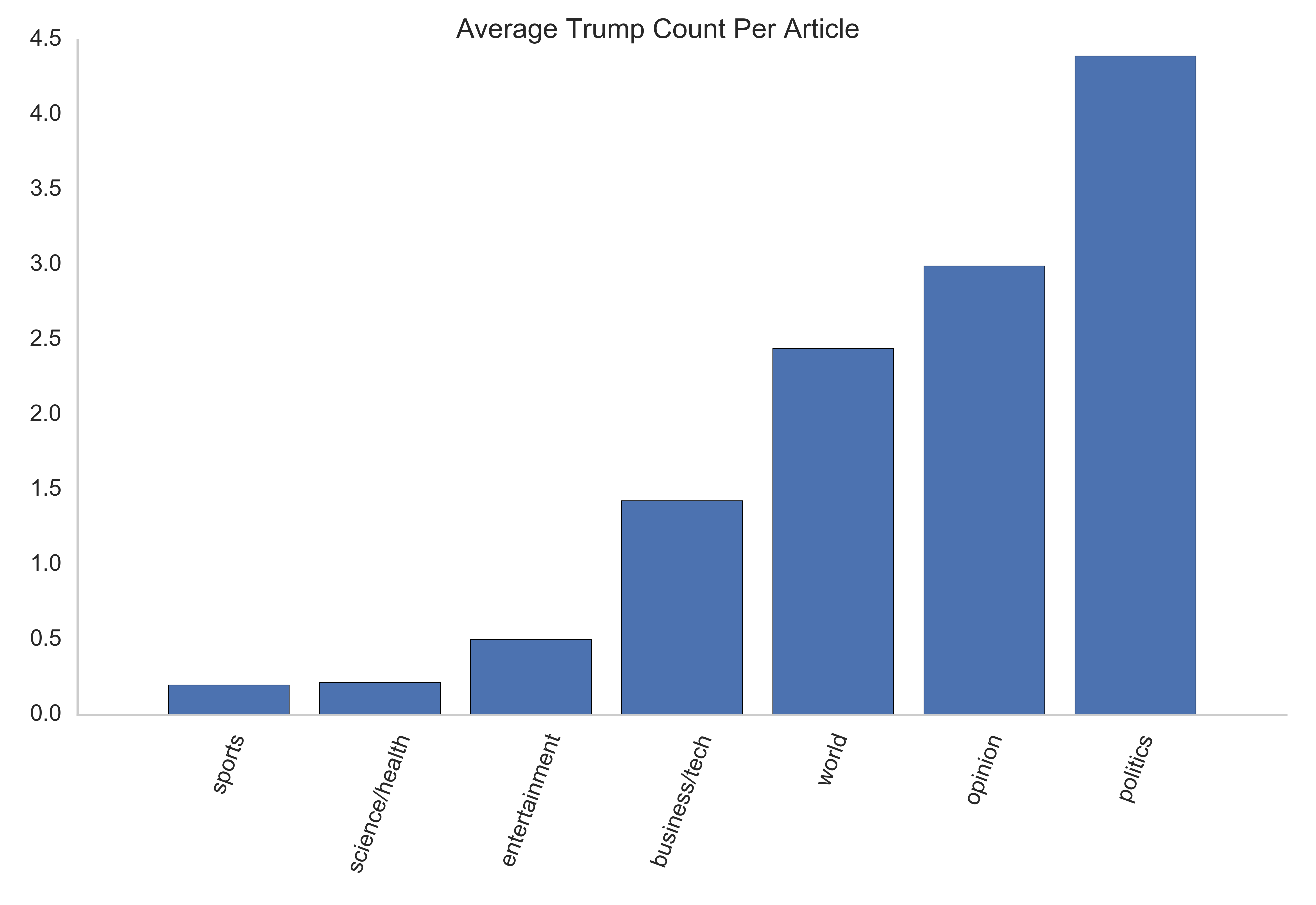
This graph really demonstrates how ubiquitous Trump is in the news. He averages 4.5 mentions per politics article, and even half a mention per science/health article. The second most commonly mentioned people were Obama (politics and opinion), Peter Thiel (the inventor of Paypal, business/technology), Andrew Rosenberg (Union of Concerned Scientists, science/health) and “Kim” (world news). One of the flaws in my processing pipeline is that words are tokenized into unigrams before being tagged by the Name Entity Recognizer, so first and last names are split. Given that “Jong” was the number three most common name in world news, I can infer that this Kim refers to Kim Jong Un or Kim Jong Il, rather than Kardashian, but the number two mention in entertainment, “David” is less clear. The upside of tagging only unigrams is that I learned that the entertainment section refers to people by their first names more commonly than other sections, as many of the top twenty most common people were first names.
Plotting with HighCharts
I thought it might be interesting to plot the fluctuation in sentiment of a particular topic over time. The SentimentPlotter class extracts all scores of articles mentioning a topic for the selected source and section, and returns them as Javascript arrays ready for insertion into a Highcharts script. The resulting graph shows the mean score for articles by day, as well as error bars for the minimum and maximum scores on that day. Mousing over the end of an error bar will reveal the title of the article that earned the high or low score. In addition the plot_topic function does the same thing, but produces a static image using the Seaborn plotting library.
#!/usr/bin/env python

import numpy as np
import pandas as pd
import json
from sqlalchemy import create_engine
from datetime import datetime, timedelta
import psycopg2
import seaborn as sns
import matplotlib.pyplot as plt
from nltk.sentiment.util import *
from nltk.corpus import sentiwordnet as swn
from nltk.tag.perceptron import PerceptronTagger
from nltk.tag import StanfordNERTagger
from nltk.tokenize import word_tokenize
import os
import re

class SentimentPlotter():
    def __init__(self, data = None):
        self.data = data

    def call(self):

        self.data['SA_body'] = [self.compute_score(x) for x in self.data['body']]
        self.data['SA_title'] = [self.compute_score(x) for x in self.data['title']]

        return self

    def get_highcharts_series(self, section = None, source = None, topic = None, date = None):
        self.section = section
        self.source = source
        self.topic = topic
        self.date = date

        self.range_date_dict, self.groupings = self.make_dict()

        self.x_dates, self.y_means, self.error_pairs, self.date_list = self.get_plotting_data()

        self.spline_series = self.get_spline_series()

        self.error_bar_series = self.get_error_bar_series()

        self.min_titles, self.max_titles = self.get_titles()

        self.min_scatter_series, self.max_scatter_series = self.get_scatter_points()

        return self.spline_series, self.error_bar_series, self.min_scatter_series, self.max_scatter_series


    def compute_score(self, sentence):
        tagger = PerceptronTagger()
        taggedsentence = []
        sent_score = []
        taggedsentence.append(tagger.tag(sentence.split()))
        wnl = nltk.WordNetLemmatizer()
        for idx, words in enumerate(taggedsentence):
            for idx2, t in enumerate(words):
                newtag = ''
                lemmatizedsent = wnl.lemmatize(t[0])
                if t[1].startswith('NN'):
                    newtag = 'n'
                elif t[1].startswith('JJ'):
                    newtag = 'a'
                elif t[1].startswith('V'):
                    newtag = 'v'
                elif t[1].startswith('R'):
                    newtag = 'r'
                else:
                    newtag = ''
                if (newtag != ''):
                    synsets = list(swn.senti_synsets(lemmatizedsent, newtag))
                    score = 0.0
                    if (len(synsets) > 0):
                        for syn in synsets:
                            score += syn.pos_score() - syn.neg_score()
                        sent_score.append(score / len(synsets))
            if (len(sent_score)==0 or len(sent_score)==1):
                return (float(0.0))
            else:
                return (sum([word_score for word_score in sent_score]) / (len(sent_score)))


    def make_dict(self):
        # define masks
        section_mask = (self.data['condensed_section'] == self.section)
        source_mask = (self.data['source'] == self.source)
        date_mask = (self.data['date'] > self.date)

        # initialize lists for range_date_dict
        topic_scores = []
        dates = []
        groupings = []

        # initialize dict
        range_date_dict = {}

        if not self.date:
            print "Please select a start date."

        # make plot_date_dict from appropriate subset of data
        else:
            if self.section and self.source:
                masked_data = self.data[section_mask & source_mask & date_mask]

            elif self.section and (not self.source):
                masked_data = self.data[section_mask & date_mask]

            elif self.source and (not self.section):
                masked_data = self.data[source_mask & date_mask]

            else:
                masked_data = self.data[date_mask]

            for i, row in masked_data.iterrows():

                if self.topic in row[2]:
                    topic_scores.append(row[6]) #body score
                    dates.append(row[1])
                    # score_title_date is tuple containing the title, date, and score
                    score_title_date = (row[0], row[1], row[6])
                    #groupings is a list of all the tuples
                    groupings.append(score_title_date)


                    # add to range_date_dict where keys are the dates and the values are a list of scores
                    if row[1] not in range_date_dict.keys():
                        range_date_dict[row[1]] = [row[6]]

                    elif row[1] in range_date_dict.keys():
                        (range_date_dict[row[1]]).append(row[6])

        return range_date_dict, groupings


    def get_plotting_data(self):
        # get dates for x-axis
        date_list = self.range_date_dict.keys()
        date_list.sort()
        # format date for javascript
        x_dates = [x.value// 10 ** 6 for x in date_list]

        # y-values
        y_values = [np.mean(self.range_date_dict[x]) for x in date_list] # mean score for the spline series

        # error bars
        error_min_max = []
        for x in date_list:
            temp_list = []
            minimum = min(self.range_date_dict[x])
            maximum = max(self.range_date_dict[x])
            temp_list.append(minimum)
            temp_list.append(maximum)
            error_min_max.append(temp_list) #error_min_max is a list of lists containing minimum and maximum

        return x_dates, y_values, error_min_max, date_list

    def get_spline_series(self):
        # format splines for Highcharts
        d = []
        series = {'name': 'Mean Score', 'type': 'spline'}
        for x in range(len(self.date_list)):
            data_point = [self.x_dates[x], self.y_means[x]]
            d.append(data_point)
        series['data'] = d
        spline_series = json.dumps(series)
        return spline_series

    def get_error_bar_series(self):
        d = []
        series = {'color': '#FF0000', 'name': 'Range', 'type': 'errorbar', 'stemWidth': 3, 'whiskerLength': 0}
        for x in range(len(self.date_list)):
            data_point = [self.x_dates[x], self.error_pairs[x][0], self.error_pairs[x][1]]
            d.append(data_point)
        series['data'] = d
        error_series = json.dumps(series)
        return error_series

    def get_titles(self):
        min_score_titles = {}
        max_score_titles = {}

        # min scores
        for x in self.groupings:
            if x[1] not in min_score_titles.keys():
                min_score_titles[x[1]] = (x[2], x[0])
            elif x[1] in min_score_titles.keys():
                if x[2] < min_score_titles[x[1]][0]:
                    min_score_titles[x[1]] = (x[2], x[0])
                elif x[2] >= min_score_titles[x[1]][0]:
                    continue

        # max scores
        for x in self.groupings:
            if x[1] not in max_score_titles.keys():
                max_score_titles[x[1]] = (x[2], x[0])
            elif x[1] in max_score_titles.keys():
                if x[2] > max_score_titles[x[1]][0]:
                    max_score_titles[x[1]] = (x[2], x[0])
                elif x[2] <= max_score_titles[x[1]][0]:
                    continue

        min_titles = [min_score_titles[x][1].encode('ascii', 'ignore') for x in self.date_list]
        max_titles = [max_score_titles[x][1].encode('ascii','ignore') for x in self.date_list]

        return min_titles, max_titles

    def get_scatter_points(self):
        max_series = []

        for x in range(len(self.date_list)):
            data_point = {'showInLegend': False, 'type': 'scatter', 'color': '#FF0000',
                          'marker': {'symbol': 'circle', 'enabled': True, 'color': '#FF0000'},
                          'tooltip': {'pointFormat': '{point.y}'}}

            data_point['name'] = self.max_titles[x]

            data_list = [[self.x_dates[x], self.error_pairs[x][1]]]

            data_point['data'] = data_list
            max_series.append(data_point)

        max_series = json.dumps(max_series)

        # return minimum scatter points series
        min_series = []

        for x in range(len(self.date_list)):
            data_point = {'showInLegend': False, 'type': 'scatter', 'color': '#FF0000',
                          'marker': {'symbol': 'circle', 'enabled': True, 'color': '#FF0000'},
                          'tooltip': {'pointFormat': '{point.y}'}}
            # get title
            data_point['name'] = self.min_titles[x]

            data_list = [[self.x_dates[x], self.error_pairs[x][0]]]

            data_point['data'] = data_list

            min_series.append(data_point)

        min_series = json.dumps(min_series)

        return min_series, max_series

    def plot_topic(self, topic = None, section = None, source = None, date = None):
        self.topic = topic
        self.section = section
        self.source = source
        self.date = date

        self.range_date_dict, self.groupings = self.make_dict()

        x = self.range_date_dict.keys()
        x.sort()
        ordered_x = []
        y = []
        for val in x:
            ordered_x.append(val)
            values = self.range_date_dict[val]
            mean = np.mean(values)
            y.append(mean)

        # define upper and lower boundaries for error bars
        upper_bounds = [max(self.range_date_dict[x]) for x in ordered_x]
        lower_bounds = [min(self.range_date_dict[x]) for x in ordered_x]

        # define distance for upper error bar
        y_upper = zip(y, upper_bounds)
        upper_error = [abs(pair[0] - pair[1]) for pair in y_upper]

        # define distance for lower error bar
        y_lower = zip(y, lower_bounds)
        lower_error = [abs(pair[0] - pair[1]) for pair in y_lower]

        asymmetric_error = [lower_error, upper_error]

        plt.plot(ordered_x, y, c = 'r', marker = 'o')
        plt.errorbar(ordered_x, y, yerr = asymmetric_error, ecolor = 'r', capthick = 1)
        plt.xlim(min(ordered_x) + timedelta(days = -1), max(ordered_x) + timedelta(days = 1))
        plt.xticks(rotation = 70)
        plt.show()
# Example of plot_topic
sp.plot_topic(topic = 'Ivanka', date = datetime(2017,1,1))

Feature Selection
Since the TfidfVectorizer yielded approximately 119,000 unigrams and bigrams, feature reduction was a necessity. Every unique word in a document can represent a new feature, so it’s important to identify which words are the most informative and train a model on those, discarding the less informative words in order to reduce dimensionality and save time transforming data and fitting models. In addition, having a set vocabulary allows a classifier to work on new articles that may contain words it’s never seen before. Since the news reports on new topics daily, this vocabulary would have to be continuously updated and optimized to account for content drift over time and to maintain a high level of accuracy.
PCA
I tried a Principal Component Analysis and found that 80% of variance in the data could be explained with around 500 principal components, and over 90% could be explained with 800 principal components. However, when I fit a Naive Bayes classifier using 800 principal components, accuracy was only 56%. This low score, plus the loss of interpretability of the principal components made PCA less appealing than other dimensionality reduction methods.

SelectKBest
The chi2 criterion is useful in feature selection for text classification tasks [3], so I compared the performance of Scikit-Learn’s SelectKBest selector with k ranging from 100 to the full feature set with the chi2 scoring function, and assessed performance using a Bernoulli Naive Bayes classifier. Accuracy began to plateau with around 5000 features, so I built a vocabulary based on the top 5000 most informative features.

This table lists the 15 most informative unigrams and bigrams, sorted by p-value. The chi2 score function assesses how unlikely the existing Tf-Idf scores would be if terms were distributed among the newspaper sections by chance. The most section-specific terms seem to be sports-related, though “researcher” and “company” may be specific to the science/health and business/tech sections respectively.

Pipeline
This pipeline can be used to format new articles for classification. It includes all necessary transformations on an ArticleData object, as well as a scaling step. However, the entire pipeline does not preserve column names, so it is unfit for exploratory data analysis. If column names need to be preserved, TitleTransformer and BodyTransformer can be applied separately, and their results concatenated with the ‘condensed_section’ column for analysis.
ItemSelector
TitleTransformer and BodyTransformer are written to only perform operations on the ‘title’ and ‘body’ columns of an ArticleData object. However, since the TfidfVectorizer need only be applied to the article bodies, I needed another transformer that could select a particular column and pass it on. ItemSelector can be combined with another more general Transformer in a sub-pipeline to apply a transformation to a subset of the total data.
class ItemSelector(BaseEstimator, TransformerMixin):
    def __init__(self, key):
        self.key = key

    def fit(self, X, y = None):
        return self

    def transform(self,X):
        return(X[self.key])
The Complete Pipeline
All features are derived and combined in a FeatureUnion during the ‘features’ step: applying title and body transformations, Tf-Idf vectorizing with a vocabulary of the top 5000 words derived from K-Best selection (‘bigram_vocab’), and a transformation to dense.
from sklearn.preprocessing import MinMaxScaler
from sklearn.pipeline import Pipeline, FeatureUnion
from sklearn.base import TransformerMixin, BaseEstimator
from mlxtend.preprocessing import DenseTransformer

pipe = Pipeline([('features', FeatureUnion([('t',TitleTransformer()),
                                            ('b', BodyTransformer()),
                                            ('tf-pipe', Pipeline([
                                            ('items', ItemSelector(key = 'body')),
                                           ('tfidf', TfidfVectorizer(preprocessor = tokenize, ngram_range = (1,2),
                                                                     min_df = 10, vocabulary = bigram_vocab)),
                                           ('dense', DenseTransformer())]))
                    ])),
                 ('scale', MinMaxScaler())
                 ])

# use fit_transform to prepare data for model fitting
# Warning: takes several hours to run for 4000 articles
Xt = pipe.fit_transform(data)
Models
Naive Bayes are the go-to models for text classification tasks, as they are reasonably efficient and robust to errors, especially when the sample size is relatively small [1]. However, other viable options include decision trees, K-Nearest Neighbors, and Support Vector Machines.
I tested six models in total using Scikit-Learn: KNN (with k ranging from 5-50, here reporting the highest score at k = 10), a random forest classifier, Adaboost, SGDClassifier, BernoulliNB, and MultinomialNB.
I witheld 30% of the data as a test set, and used a 5-fold cross-validated grid search to optimize hyperparameters for each model. The top two performers were Bernoulli Naive Bayes and Stochastic Gradient Descent Classifier at about 85% accuracy each. Interestingly, Multinomial Naive Bayes performed the worst, at only 32% accuracy. Multinomial Naive Bayes differs from Bernoulli Naive Bayes in that it assumes positional independence of tokens, which the data almost certainly violates, as words in written language have a meaningful and non-random sequence.

Model Evaluation
The confusion matrices for the two top-performing models contain diagonal bands of high values indicating the correctly categorized articles. The most difficult section to classify appears to be business/technology, as it has the lowest f1-score for both classifiers, though the SGDClassifier slightly out-performs the Naive Bayes. The opinion section also appears to pose some challenges for both classifiers, as both have low recall scores for this section, meaning that many opinion pieces are misclassified into other sections. This seems like a natural mistake to make, as an opinion piece could be written about any topic, and therefore, topical feature words might be less informative.
However, it’s worth noting that the Naive Bayes model runs much, much faster than the SGDClassifier (a matter of minutes rather than hours).
Bernoulli Naive Bayes


SGDClassifier


For the SGDClassifier, I investigated the coefficient matrix to see which terms were the most informative for each class. This bubble chart shows the most features with the highest positive coefficient for each section. The sports section is defined strongly by terms like ‘game’, ‘injury’, or ‘team’, while the entertainment section is defined by ‘novel’, ‘performance’, or the number of people in the article title. Interestingly, opinion articles frequently the terms ‘read post’ or ‘read topic’, which may indicate that they are responses to other articles.
Learning Curves
To investigate whether or not the classifiers might benefit from more data, I plotted the learning curves of the Bernoulli Naive Bayes and the SGDClassifiers. The training and cross-validation scores of the Naives Bayes classifier seem to be converging around 85%, so this model may not improve much with a larger sample size, but might benefit from further feature engineering.
from sklearn.learning_curve import learning_curve
from sklearn.cross_validation import ShuffleSplit

cv = ShuffleSplit(n = 10, test_size = 0.3)
train_sizes, train_scores, valid_scores = learning_curve(sgd_model, X_select, y, cv = cv)

train_scores_mean = np.mean(train_scores, axis = 1)
test_scores_mean = np.mean(valid_scores, axis = 1)

However, the cross-validation score of the SGDClassifier does not seem to have plateaued at 4,000 samples, and may improve with more data.

Conclusions and Future Directions
This analysis has yielded two models that can classify a news article into the appropriate newspaper section with 85% accuracy. The primary use case for these classifiers is for online publishers or aggregators of news stories to tag articles for easy searching or sorting, though they might also be useful to archivists, librarians, or any other business seeking to organize and categorize text.
There are several improvements that could be made to the classification process. Learning curves indicated that the Stochastic Gradient Descent classifier would benefit from a larger corpus, which is easily obtainable through web-scraping. In addition, including word counts from Scikit-Learn’s CountVectorizer or counts of percents, dates, or numbers from a more complex Named-Entity Recognizer might help to boost accuracy for both SGDClassifier and Bernoulli Naive Bayes.
However, including these features and more data would add processing time to an already slow transformation pipeline, so parallelizing this process on a framework like Spark or Hadoop would greatly facilitate the speed at which predictions could be made.
References
[1] Manning, C.D., Raghavan, P., Schutze, H. 2009. Introduction to Information Retrieval Online Edition. Cambridge (UK). Cambridge University Press.
[2] Bengfort, Ben. Text Classification with NLTK and Scikit-Learn. Blog Post. Libelli, 19 May 2016. Web. Accessed 2017.
[3] Fuka, K, Hanka, R. (2001). Feature Set Reduction for Document Classification Problems. Conference Proceedings. IJCAI-01 Workshop: Text Learning: Beyond Supervision. Seattle. University of Cambridge.